Selecting an embedded MCU for SoC

This is a guest post by Dolphin Integration which provides IP core, EDA tool and ASIC/SoC design services

When a SoC integrator has to select a microcontroller for his application, most of the time, he refers to his own previous experiences rather than on a rational assessment as no standard benchmarking process has emerged for selecting an embedded microcontroller. The reason is that there are a lot of criteria to consider and it is difficult to achieve a fair comparison between the different products available.

Experience shows that the main criteria to consider when selecting a microcontroller are, on one hand: speed, area, consumption, computing power, code density, on the other hand: quality and maturity of development & debug tools. Each of these criteria depends on many parameters and conditions for evaluation that make accurate comparisons difficult. Moreover, the selection of an embedded MCU requires that the evaluator knows how to balance the relative value of each criteria depending on the challenges of the top circuit implementation.

Therefore, due to the complexity of parameters to be taken into account (technology, Process/Voltage/Temperature conditions, standard cell library, tools versions …), and knowing that it is rare that suppliers provide exhaustive specifications of all these parameters when communicating the performances of a core, it is unlikely that the evaluator can make a meaningful comparison between different products based only on data given in the datasheets. In this article we will discuss the pitfalls to avoid during the assessment of the relevant criteria for the selection of an embedded MCU, and we will propose some guidelines to make such assessments more straight forward.

POWER CONSUMPTION

Indeed, the power consumption of a processor depends on many factors such as the target technology (lithography size, process flavour, threshold voltages…see Table 1), the library of standard cells used to implement the core and the execution activity imposed on the processor during power simulation. Beyond that, what is left unsaid is often more important than what is stated explicitly. Consequently, caution and judicious reading of the vendor data sheets are mandatory when comparing the power figures for competing processor IP. Rarely, you will find apples to compare with apples from the data sheets only.

Table 1: Process option versus Power

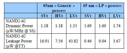
The table 1 shows the great variability of power according to threshold voltages and process variant. In the given example (NAND2 drive 2 gate), the dynamic power can be 43 % higher in LP process but the leakage power can be up to 175 times lower! Furthermore, as leakage varies dramatically with temperature, letting the reader unaware of the process and temperature corner being used for power estimation may lead to a wrong comparison and then to attribute artificial qualities to a processor. Table 2 shows the impact of standard cells library selection on power figures: depending on the library chosen in the same lithography and the same process, the dynamic power may vary in a wide proportion.

Table 2: Library options versus Power

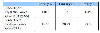
Figure 1 shows the impact of process corner on power specifications. We can notice that the PVT conditions applied for the measurement can decrease of 30% the power consumption

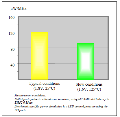
Figure 1: Flip80251-Typhoon power consumption in different PVT conditions

While values of power consumption of a packaged processor (standard chip) take necessarily into account all circuitry in the package, power specifications of processor cores are based on simulations – vendors are free to delete or ignore any number of power-dissipating functions when reporting power numbers. Some vendors do not include specific functions when they measure the power consumption. They often specify in their datasheets what they did not take into account.

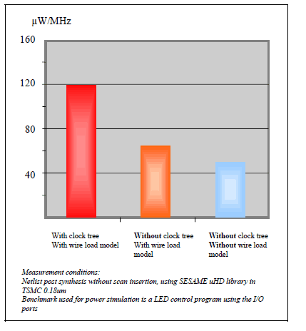
However, sometimes, these functions are vital for the microcontroller. For example, when a supplier does not include the clock tree, the customer has to appreciate the consequences of this omission: indeed, the clock tree includes the gates operating at the highest frequency of the core. This function dissipates much of the CPU power. It is not possible to design a microcontroller without clock tree. Obviously, it would be unfair to compare the power specifications of two processors and omit the clock tree from one of them (see Figure 2).

Figure 2: Flip80251-Typhoon power consumption with/without function omission

Another example of frequent omission: Shall we consider the static consumption? It will depend on the fabrication technology, the Vt flavour selected (i.e. Nominal, High or Low Vt), the temperature range and the operating frequency. Indeed, down to 180 nm technology, static power consumption is not considered because it is insignificant compared to the dynamic power consumption. However, in advanced fabrication technology, from 90 nm and beyond, the static power consumption cannot be ignored anymore. It could represent a significant part of the total consumption but most of the time, vendors do not indicate the static power consumption.

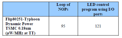
Even if the datasheet clarifies all the items listed above, one more important “detail” remains unclear (in most of the datasheet): What is the processor doing while the power simulations run? If the program being run during the power simulation is a loop of NOPs (i.e. no operation), the customer would expect to get lower power numbers than if the processor were exercising its function units. Thus even the benchmark program being run during power simulation can influence the core’s power consumption specifications.

Table 3: Influence of processor activity on power figures

Data contained in datasheets will give a global idea of the dynamic consumption. Thanks to that, it will help to have an overview of the consumption of competitors’ solutions, but since no standardized power-benchmarking program for processor cores has emerged and since the measurement conditions can be far from the customer’s application conditions, it seems unrealistic to have accurate power consumption estimation for a microcontroller without running its own power simulations.

Thus, such partial data will not enable an accurate model of the consumption, which is essential to the SoC designer for proper sizing of the power grid to meet IR-drop and Electro-Migration criteria. We encourage the customer to run his own power simulation for two reasons. He could have a full control of the evaluation conditions and he could assess the power consumption of the rest-of-SoC, especially the memory system, in the mean time.

This last point is important and often underestimated: an embedded processor is just one part of the system and a processor that enables to reduce the number of access to the memory system is a better processor for low power optimisation. So, it is important to use EDA solutions to have an early assessment of the system power consumption. When evaluating a processor core, you could benefit from an evaluation version of our SCROOGE EDA solution. It enables to get quickly an accurate estimation of the power consumption thanks to the emulation of the clock tree and the wire loads.

AREA

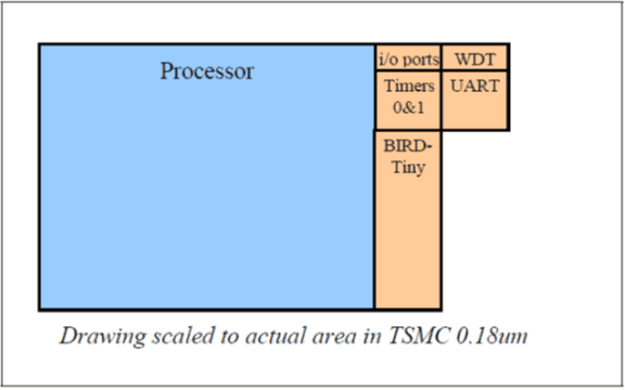
When processor vendors communicate on the area, there are also some omissions that could make the numbers meaningless. The MCU area depends a lot on the configuration considered: is it only the processor configuration? If not, which peripherals are considered? Which options? These questions are really crucial when considering the MCU area. For example the MCU Flip80251 Typhoon with the processor configuration is raised by 24% adding standard peripherals like Timers, UART, I/O ports and an embedded debug support (see Figure 3). The difference of areas can be very significant between the configurations. As a result, to compare the area of two MCUs, their configurations have to be purely the same. Even some synthesis options like scan insertion have to be considered or not in the area estimation and indicated in the measurement conditions.

Figure 3: Flip80251-Typhoon area

Core vendors are used to communicate on area either in terms of number of (equivalent) gates or by giving a silicon area in mm2. Both ways present some traps to avoid.

The number of gates is helpful to express the area independently of the library chosen for the synthesis. It is computed by dividing the core area after synthesis by the area of a reference gate. For all vendors, this reference gate is a NAND2 gate, but is there only one NAND2 gate? The answer is no because there are different subtypes of NAND2 gates varying in size. A NAND2 gate is available in several “drives” in a library: for instance, a NAND2-drive1 has an area of 7.526 μm2 in TSMC 0.18 μm process, and a NAND2-drive2 has an area of 15 μm2. As a result, an IP of 5,000 gates for NAND2-drive1 equivalent Gate count will be announced at 2,500 gates for NAND2-drive2 equivalent Gate count. So, the figure is very different from one count to another if the drive is not indicated in the IP supplier documentation.

The other point that makes the gate count comparison unfair is the variability of gate size between libraries. The relative size between the NAND2 and the others cells has a direct impact on the gate count. Imagine you are synthesizing a core with 2 libraries in TSMC 0.18um which differs only for the size of the NAND2 drive 1 and the size of one Flip-Flop. The library A has a NAND2 of 10 um2 and a DFF of 100 um2. The library B has a larger NAND2 (15 um2) but a smaller DFF (95 um2). Suppose that for a given design, the number of NAND2 and DFF is the same. The total area would be identical with library A and library B. However, the library A will give a gate count 50% Processor i/o ports WDT Timers 0&1 UART BIRDTiny Drawing scaled to actual area in TSMC 0.18um  larger than the library B even if it is the same core, synthesized with the same constraint in the same technology. As a result, the gate count depends on multiple parameters. It can be drastically different depending on how it is calculated and what is considered. The gate count is uncertain and so, not significant to conclude on the MCU area.

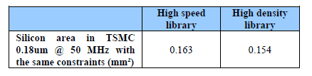
Therefore, the silicon area is the figure that really matters. It will represent the real cost for the designer and its customer. However, once again, this figure depends on many parameters: the lithography size and the process, the standard cells library used, the PVT conditions, the synthesis constraints (frequency, I/O delays, max cap, rest of SoC constraints, etc…), and if the result is pre or post place and route. Taking into account all these parameters, it seems impossible to compare area figures from different providers measured in exactly the same conditions. The customer will even have to ask to the MCU provider to give the detailed measurement conditions because it is rarely indicated in the datasheets. Then, the figure of the datasheets will be useful for a first evaluation.

Table 4: Influence of library in core area

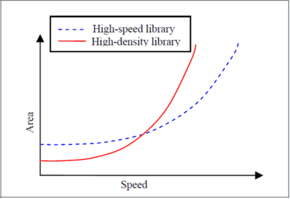
Moreover the principal parameter impacting the area is the clock frequency chosen. Between area oriented optimization and speed-oriented optimization synthesis, the result will be widely different. It demonstrates that this information is crucial when comparing value in data sheet, to know if the microcontrollers are compared in the same conditions.

Figure 4: impact of target speed on silicon area

As a conclusion, if a SoC designer wants to get, from the datasheets, some information about the MCU area, he will have to be very careful on the measurement conditions. But he has to keep in mind that for tiny processors in advanced technological processes, the CPU area is so minimized and the difference would be so small that the gate count should be a secondary decisive factor.

SPEED

As shown before, even if the frequency and the area are highly linked together, the right way to define target frequency is to look at the frequency that enables to process the critical part of the application program in the required amount of time. Then, you could assess what is the impact of the required frequency on area and power. Indeed, the goal is not to target the highest frequency possible with a core because it would give both a huge area and a high consumption, but to find the pair “processing power – core frequency” that provides the best trade-off area / power. In that way, processor frequency has to be considered rather as a trade-off that enables to achieve the others target. In the next chapter, we will propose a method to assess the processing power needed avoiding the classical traps.

CODE DENSITY / PROCESSING POWER

The wide range of applications makes it difficult to characterize the embedded domain. In embedded systems, the applications range from sensor systems with simple MCUs to smart phones that have almost the functionality of a desktop machine combined with support for wireless communications. Another particularity of the embedded world is that there is not a significant legacy code base that would favour a standard instruction set architecture (ISA), as it has happened in the desktop world. This has led to a remarkable diversity of ISAs for embedded applications that makes the selection of the benchmark program even more crucial for finding the best architecture for a particular application. The more frequent pitfall when evaluating the code density or the processing power is to underestimate the role of the selected benchmark on the reliability of the result. By not applying the right benchmark, you could select a processor which is not the most appropriate for your application as shown in the table 5 below.

Table 5: Code size for different benchmark

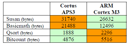
These benchmarks are part of the category “industrial control” of MiBench.

So, the question is: how to select the right benchmark for a meaningful appreciation of the processing power (and consequently the code density)?

Since different application domains have different execution characteristics, a wide range of benchmark programs has been developed in the attempt to characterize these different domains. Most of these benchmarks are targeted towards specific areas of computation. For instance, the primary focus of the Dhrystone was to measure integer performance; LINPACK is for vectorizable computations; and Whetstone is for floating point intensive applications. Other benchmarks are available to stress network TCP/IP stacks, data input/output and other specific tasks.

Even if the limitations of Dhrystone are well known by a majority of developers, Core vendors, including the largest one, ARM™, are still communicating on processor performance by giving their Dhrystone score.

Why Dhrystone is not good?

The Dhrystone is a “synthetic benchmark”. Synthetic benchmark programs are artificial programs that include mixes of operations carefully chosen to match the relative mix of operations observed in some class of applications programs. The hypothesis is that the instructions mix is the same as those of the user program, so that the performance obtained when executing the synthetic program should provide an accurate indication of what would be obtained when executing an actual application. The main problem is that the patterns, for memory access in real application, are very hard to duplicate in a synthetic program. These patterns determine memory locality that deeply affects the performance of a hierarchical memory subsystem (i.e. including a cache). As a result, hardware and compilation optimization can produce execution times that are significantly different that the execution times produced on actual application programs, even though the relative instructions mix is the same in both cases.

To improve the limited capabilities of synthetic benchmarks, standardized sets of real application programs have been collected into various application-program benchmark suites. These real application programs can more accurate characterize how current applications will exercise a system than the other types of benchmark programs. However, to reduce the time required to run the entire set of programs, they often use artificially small input data sets. This constraint may limit the ability of the application to accurately model the memory behavior and I/O requirements of a user’s application programs. However, even with these limitations, these types of benchmark programs are the best to been developed to date.

There have been some efforts to characterize embedded workloads, most notably the suite developed by the EEMBC consortium and its academic equivalent MiBench. They have recognized the difficulty of using just one suite to characterize such a diverse application domain and have instead produced a set of suites that typify workloads in some embedded markets. For instance, MiBench benchmark programs are divided into six suites with each suite targeting a specific area of the embedded market. The categories are Automotive and Industrial Control, Consumer Devices, Office Automation, Networking, Security, and Telecommunications. All the programs are available as standard C source code for being portable.

It is important to note that a benchmark program should be easy of use and should be relatively simple to execute on a variety of systems. A benchmark difficult to use is more likely to be used incorrectly. Furthermore, if it is not easy to port the benchmark to various systems, it is probably a better use of the performance analyst’s time to measure the actual application performance instead of spending time trying to run the benchmark program.

In summary:

• Select carefully your benchmark according to your application domain
• Do not blindly trust the result if you are not able to clearly state how close of your real application the benchmark program is
• Do not underestimate the capacity to optimize a C code for a given architecture. If the evaluator is porting a C code that has been optimized for a different architecture, it is likely that the first density resulting on the new architecture is far from the best result that can be achieved with this architecture. Furthermore, take care of the relative Ccompiler optimization
• Take care of C-library support / optimisation. Most of the recent 32-bit MCU architectures have a development tools suite based on GCC. The C-library of GCC includes support of functions that are most of the time useless in embedded systems. As a result, if these libraries are not optimised for embedded system, they will be unnecessary large. Optimizing C library is a way to reduce code size without modifying application program or optimizing C compiler

CONCLUSION

It is very easy to make a processor assessment that leads to a wrong conclusion, because at each step of the evaluation, there are many possibilities to compare data that where not measured under the same conditions. That is the reason why we could see many circuits that embeds not the most appropriate MCU, but only a convenient one. In this article, we have seen how Dolphin documents a rigorous frame that enables to avoid the main pitfalls of the evaluation process and, when coupled with advanced power-simulation tools and methodologies leads to an objective assessment of different MCU architectures to select the right embedded MCU for the targeted application.

Click here to learn more about Dolphin Integration products and services

.